Preprocessing iNaturalist data

This section covers:

Download iNaturalist ‘research-grade’ vasuclar plant observations
iNaturalist global observation density
Observation growth over the years
Frequency of observations per species

Packages¶

import pandas as pd # for handling dataframes in python
import numpy as np # array handling
import os # operating system interfaces

# packages needed for plotting:
import matplotlib.pyplot as plt # main Python plotting library 
import seaborn as sns # pretty plots
from matplotlib.colors import LogNorm, Normalize, BoundaryNorm
import cartopy.crs as ccrs # maps 
from matplotlib.ticker import MaxNLocator
from mpl_toolkits.axes_grid1 import make_axes_locatable

Download iNaturalist observation data¶

For this study we used the following download: GBIF.org (4 January 2022) GBIF Occurrence Download GBIF.Org User (2022)

If you would like to use the most recent data: Follow the above link and click ‘Rerun Query’ and proceed to download. For this analysis the ‘simple’ version is sufficient.

Load observations as data frame¶

iNat = pd.read_csv('/net/data/iNaturalist/Tracheophyta/0091819-210914110416597.csv', sep='\t')

/net/home/swolf/.conda/envs/cartopy/lib/python3.8/site-packages/IPython/core/interactiveshell.py:3172: DtypeWarning: Columns (46) have mixed types.Specify dtype option on import or set low_memory=False.
  has_raised = await self.run_ast_nodes(code_ast.body, cell_name,

iNat.head()

The dimensions of the dataframe:

iNat.shape

(14019405, 50)

The number of vascular plant species in the iNaturalist observations:

iNat["scientificName"].nunique()

103625

Extract relavent columns¶

scientificName
decimalLatitude
decimalLongitude
eventDate

iNat = iNat[["gbifID", "scientificName","decimalLatitude","decimalLongitude","eventDate", "dateIdentified"]]

Keep only the first two words of scientific name, as some names are annotated with additional information.

iNat['scientificName']  = iNat['scientificName'].apply(lambda x: ' '.join(x.split()[0:2]))

iNat.head()

Save the edited dataframe as a csv file:

iNat.to_csv("Data/iNat/observations.csv", index=False)

Density of Observations¶

We want to visualize the global distribution of iNaturalist vascualr plant observations. First, we load the observations:

iNat = pd.read_csv('Data/iNat/observations.csv')

Using the .shape function, we can have aquick look at the number of rows and colums in our dataframe.

iNat.shape

(14019405, 6)

One version of plotting the density, is by aggregating the iNaturalist observations in hexagonal bins and count the number of observations per hexagon. The function hexbin provides this functionality.

def hexmap(long, lat, label):
    
    ax = plt.subplot(projection=ccrs.PlateCarree())
    
    # add coastline outline and extent of map:
    ax.coastlines(resolution='110m', color='orange', linewidth=1)
    ax.set_extent([-180, 180, -90, 90], ccrs.PlateCarree())
    
    # hexbin aggregates observations in hexagonal bins and plots the density
    hb = ax.hexbin(long,
          lat, 
          mincnt=1, # min. nuber of observations per hexagon 
          gridsize=(100, 30), # bin size
          cmap="cool", 
          transform=ccrs.PlateCarree(), 
          bins='log', 
          extent=[-180, 180, -90, 90],
          linewidths=0.1)
    cb = fig.colorbar(hb, ax=ax, shrink=0.4)
    cb.set_label(label)

Apply the hexmap function to our iNaturalist observations and save output as .pdf:

fig = plt.figure(figsize=(10, 10))
hexmap(iNat['decimalLongitude'], iNat['decimalLatitude'], "Number of iNatrualist Observations")
plt.savefig('Figures/iNat_density_hex_tight.pdf', bbox_inches='tight')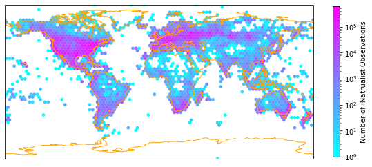

A second plotting option is to grid the data into a latitude/longitude grid. Then we can project our map onto a more realistic representation of the spherical Earth, such as the Robinson projection. The previously used hexbin function does not have a reprojection functionality implemented.

def gridmap(long, lat, label, projection, colorbar=True):
    
    plt.rcParams.update({'font.size': 15})

    Z, xedges, yedges = np.histogram2d(np.array(long,dtype=float),
                                   np.array(lat),bins = [181, 91])

    #https://stackoverflow.com/questions/67801227/color-a-2d-histogram-not-by-density-but-by-the-mean-of-a-third-column
    #https://medium.com/analytics-vidhya/custom-strava-heatmap-231267dcd084
    
    #let function know what projection provided data is in:
    data_crs = ccrs.PlateCarree()
    
    #for colorbar
    cmap = plt.get_cmap('cool')
    im_ratio = Z.shape[0]/Z.shape[1]

    #plot map
    #create base plot of a world map
    ax = fig.add_subplot(1, 1, 1, projection=projection) # I used the PlateCarree projection from cartopy
    
    # set figure to map global extent (-180,180,-90,90)
    ax.set_global()
    
    #add coastlines
    ax.coastlines(resolution='110m', color='orange', linewidth=1.3)
    
    #add grid with values
    im = ax.pcolormesh(xedges, yedges, Z.T, cmap="cool", norm=LogNorm(), transform=data_crs)
    
    #add color bar
    if colorbar==True:
        fig.colorbar(im,fraction=0.046*im_ratio, pad=0.04, shrink=0.3, location="left", label=label)

Apply the gridmap function to our iNaturalist observations and save output as .pdf. You can also experiment with other projections. See https://scitools.org.uk/cartopy/docs/v0.15/crs/projections.html for inspiration:

fig = plt.figure(figsize=(12, 12))
gridmap(iNat['decimalLongitude'], iNat['decimalLatitude'], "Number of iNatrualist Observations", ccrs.Robinson())
plt.savefig('Figures/iNat_density_Robinson_all.pdf', bbox_inches='tight')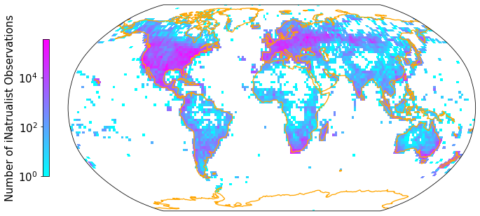

Growth of observations over time¶

The number of iNaturalist observations added every year is growing continually. Here we plot the growth of observations added every year (using the so-called “date identified”) since the iNaturalist project started in 2008.

# extract the year from 'dateIdentified':
iNat['year'] = iNat['dateIdentified'].str[:4]

def catbarplot(df, column, label):
    
    # sort dataframe by column 
    df = df.sort_values(by=[column])
    
    # white background 
    sns.set_theme(style="white")
    
    ax = sns.countplot(x=column, data=df, palette="cool",)
    
    # make remove top and right border of plot
    sns.despine()
    
    # set label text
    plt.xlabel(column)
    plt.ylabel(label) 
    
    # rotate x tick labels sightly
    ax.set_xticklabels(ax.get_xticklabels(), rotation=40, ha="right")

plt.figure(figsize=(5,5))
catbarplot(iNat, "year", "iNaturalist vascular plant observations \n added yearly in millions")
plt.savefig('Figures/iNat_growth.pdf', bbox_inches='tight')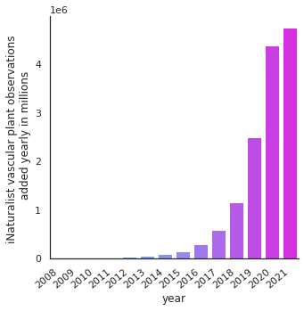

Frequency distribution of observations¶

Most species have only been observed one or two times, few species have been observed many times. The most observed species is Achillea millefolium, which has been observed 59,022 times.

species_frequencies = iNat['scientificName'].value_counts()
species_frequencies

Achillea millefolium       59022
Taraxacum officinale       47373
Trifolium repens           44175
Alliaria petiolata         43250
Trifolium pratense         39249
                           ...  
Pseudabutilon orientale        1
Ficus clusiifolia              1
Otospermum glabrum             1
Ficinia montana                1
Poa howellii                   1
Name: scientificName, Length: 90820, dtype: int64

Distribution of frequency unique species ist highly squewed. Most species are rare and few are common, as we can see in the following histogramm:

plt.hist(species_frequencies, range = (0,1000), bins=50);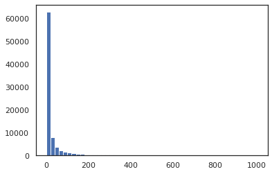

References¶

GBIF.Org User. (2022). Occurrence Download. The Global Biodiversity Information Facility. 10.15468/DL.34TJRE