Differences among biomes - Workflow library

We want to determine if the differnces between iNaturalist observations and sPlotOpen cwm’s differ across different biomes.

This section covers:

Load WWF terrestrial ecoregions and biomes
Clip observations into biomes
Calculate grid means for each biome
Visualize differences in boxplot
Quantification Average Difference

# packages
import os
import pandas as pd
import numpy as np
import os
import matplotlib.pyplot as plt
import seaborn as sns
import matplotlib.ticker as ticker
from matplotlib.colors import LogNorm, Normalize
from matplotlib.ticker import MaxNLocator
import cartopy.crs as ccrs
import cartopy.feature as cfeature
from matplotlib.colors import BoundaryNorm
import geopandas as gpd
from geopandas.tools import sjoin

Load WWF biome data¶

We use the terrestrial biomes, as defined in the WWF terrestrial ecoregion map. The WWF terrestrial ecoregions shape files were downloaded from www.worldwildlife.org/publications/terrestrial-ecoregions-of-the-world.

wwf = gpd.read_file("WWF/wwf_terr_ecos.shp")
# remove arctic and antarctica
wwf = wwf[wwf["BIOME"] < 98]

wwf.head()

Visualize biomes¶

wwf['BIOME_str'] = wwf['BIOME'].astype(str)

fig, ax = plt.subplots(figsize = (10,15))
wwf.plot(column='BIOME_str', ax=ax, cmap="tab20", legend=True);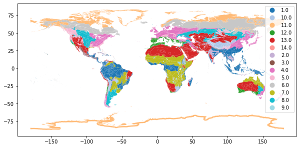

Clip observations into biomes¶

Load iNaturalist and sPlotOpen observations¶

iNat_TRY = pd.read_csv("iNat_TRY_log.csv")

sPlot = pd.read_csv("sPlotOpen/cwm_loc.csv")

# make geopandas dataframes
# projection of wwf also in epsg:4326 
geo_iNat = gpd.GeoDataFrame( iNat_TRY.iloc[:,:24], geometry=gpd.points_from_xy(iNat_TRY.decimalLongitude, iNat_TRY.decimalLatitude), 
                            crs='epsg:4326')

geo_sPlot = gpd.GeoDataFrame(sPlot, geometry=gpd.points_from_xy(sPlot.Longitude, sPlot.Latitude), crs='epsg:4326')

Clip observations¶

We use the geopandas clip() function to select the observations within the geometry of each biome:

# groupby wwf biomes
biomes = wwf.dissolve(by='BIOME')
biomes['BIOME'] = biomes.index

# clip data into biomes 
# run-time about 45 min.

iNat_with_biome = pd.DataFrame(columns=geo_iNat.columns)
iNat_with_biome['BIOME']  = []

for index, row in biomes.iterrows():
    polygon = row['geometry'] #shape of biome
    clipped = geo_iNat.clip(polygon) #select all observations within this shape
    # add biome
    clipped['BIOME'] = row['BIOME'] #add biome to corresponding observations
    iNat_with_biome = pd.concat([iNat_with_biome, clipped])

sPlot_with_biome = pd.DataFrame(columns=geo_sPlot.columns)
sPlot_with_biome['BIOME']  = []

for index, row in biomes.iterrows():
    polygon = row['geometry']
    sPlot_clipped = geo_sPlot.clip(polygon)
    # add biome
    sPlot_clipped['BIOME'] = row['BIOME']
    sPlot_with_biome = pd.concat([sPlot_with_biome, sPlot_clipped])

sPlot_with_biome.drop('geometry',axis=1).to_csv(r'sPlot_biomes.csv', index=False)

iNat_with_biome.drop('geometry',axis=1).to_csv(r'iNat_biomes.csv', index=False)

Calculate grid means for each biome¶

iNat_with_biome = pd.read_csv("iNat_biomes.csv")

sPlot_with_biome = pd.read_csv("sPlot_biomes.csv")

/net/home/swolf/.conda/envs/cartopy/lib/python3.8/site-packages/IPython/core/interactiveshell.py:3172: DtypeWarning: Columns (55) have mixed types.Specify dtype option on import or set low_memory=False.
  has_raised = await self.run_ast_nodes(code_ast.body, cell_name,

wwf = gpd.read_file("WWF/wwf_terr_ecos.shp")
# remove arctic and antarctica
wwf = wwf[wwf["BIOME"] < 98]

iNat_with_biome.head()

biome_types = sPlot_with_biome['BIOME'].unique().tolist()

def global_grid_data(df, long, lat, deg, variables):
    
    # create new dataframe to save the average value of each grid cell and variable
    grouped_df = pd.DataFrame()
    
    # convert degree into step size
    step = int((360/deg) + 1)
    
    bins_x = np.linspace(-180,180,step) 
    bins_y= np.linspace(-90,90,int(((step - 1)/2)+1))
    
    # group latitude and longitude coordinates into bins
    # create new columns 'x_bin' and 'y_bin'
    df['x_bin'] = pd.cut(df[long], bins=bins_x)
    df['y_bin'] = pd.cut(df[lat], bins=bins_y)
    
    # raster coordinates are in center of raster cell
    df['x_bin'] = df['x_bin'].apply(lambda x: ((x.left + x.right) /2) )
    df['y_bin'] = df['y_bin'].apply(lambda x: ((x.left + x.right) /2) )
    
    grouped_df = df.drop_duplicates(subset=['x_bin', 'y_bin'], keep='last')
    grouped_df = grouped_df[['x_bin', 'y_bin']]
    
    for v in variables:
        
        sub_df = df[['y_bin', 'x_bin', v]]
        grouped_v = sub_df.groupby(['x_bin', 'y_bin'], as_index=False)[v].mean()
        
        
        grouped_df = pd.merge(grouped_df, grouped_v, 
                    on= ['x_bin', 'y_bin'], 
                    how='left')
        
    return grouped_df

trait = iNat_TRY.columns[6:24]


for i in biome_types:
    
    # subset biome
    iNat_sub = iNat_with_biome[iNat_with_biome['BIOME']==i]
    sPlot_sub = sPlot_with_biome[sPlot_with_biome['BIOME']==i]
    
    # get grid means
    df_iNat = global_grid_data(iNat_sub, 'decimalLongitude', 'decimalLatitude', deg=2, variables=trait)
    df_sPlot = global_grid_data(sPlot_sub, 'Longitude', 'Latitude', deg=2, variables=trait)
    
    # reshape data, so that we have only one Trait column
    df_iNat_t = df_iNat.melt(id_vars=["x_bin", "y_bin"], 
                     value_name="TraitValue_iNat", 
                     var_name="Trait")
    
    df_sPlot_t = df_sPlot.melt(id_vars=["x_bin", "y_bin"], 
                     value_name="TraitValue_sPlot", 
                     var_name="Trait")
    
    # merge sPlot and iNat data into one dataframe
    df_merged = pd.merge(df_sPlot_t, df_iNat_t, on=["x_bin", "y_bin", "Trait"] )
    
    # keep only lines where we have a pixel in both datasets
    df_merged = df_merged.dropna()
    
    # save result to csv
    filename="WWF/grid_means_biome" + str(i) + "_2deg.csv"
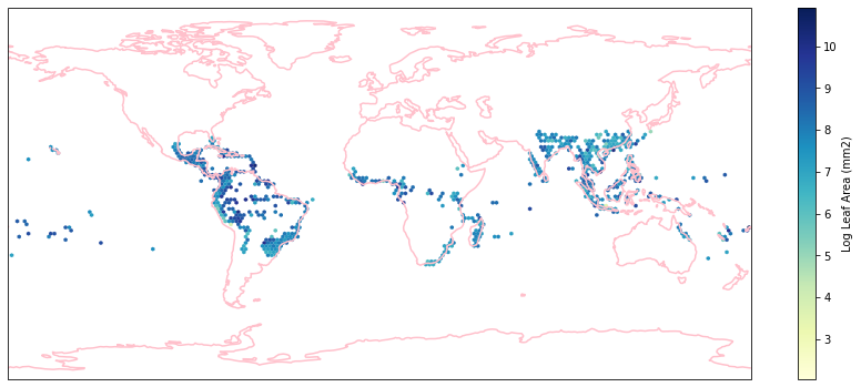
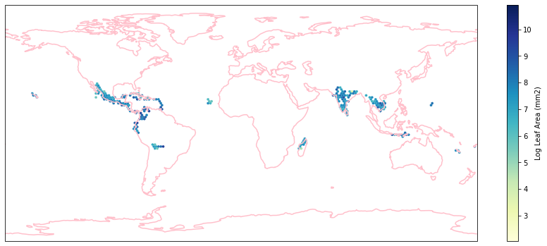
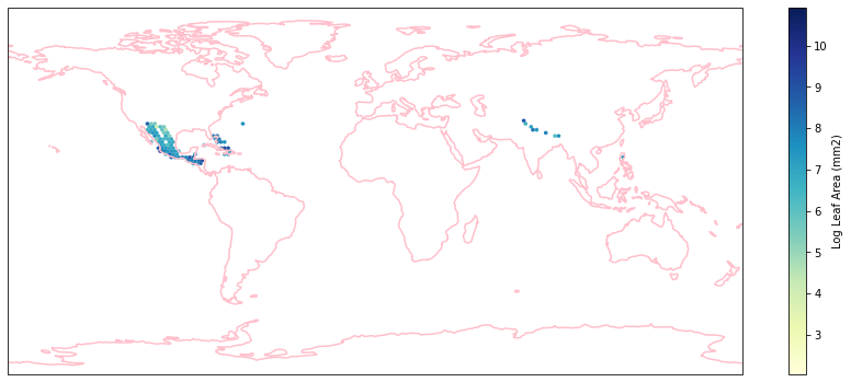
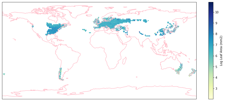
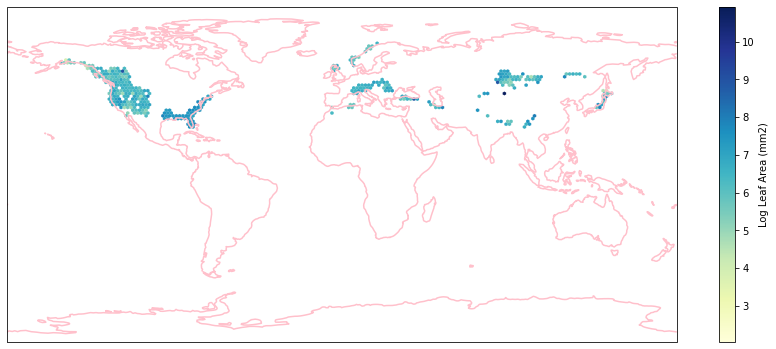
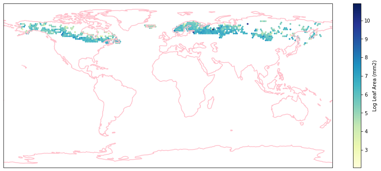
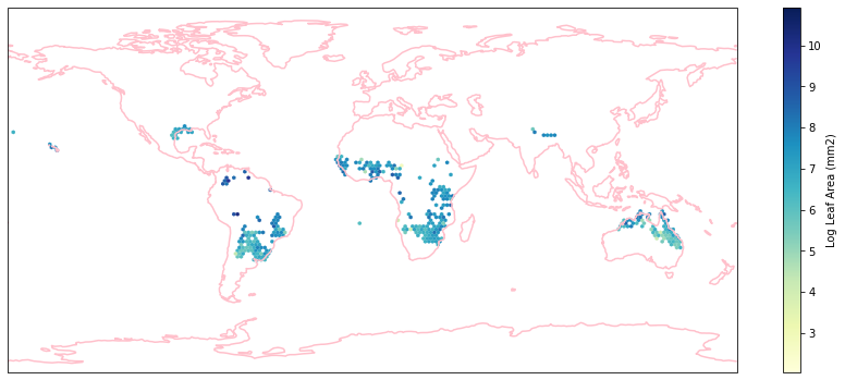
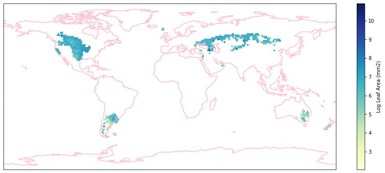
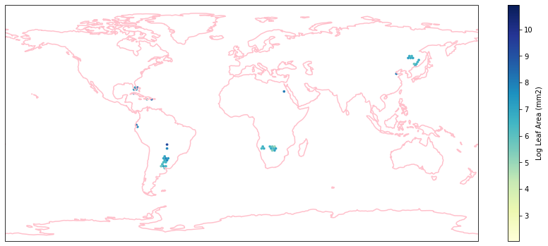
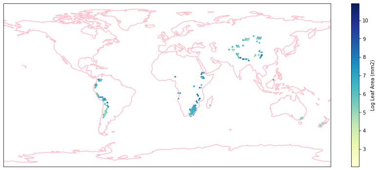
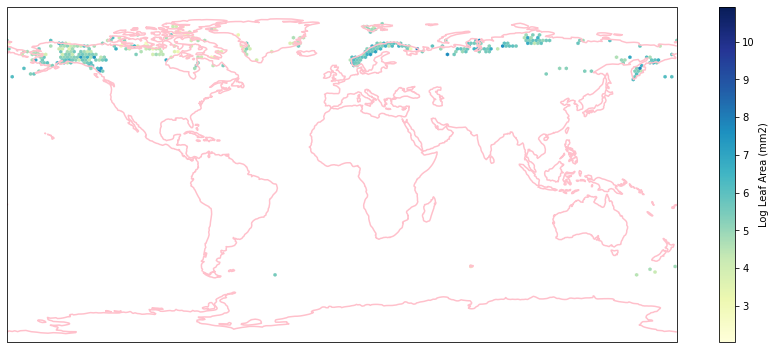
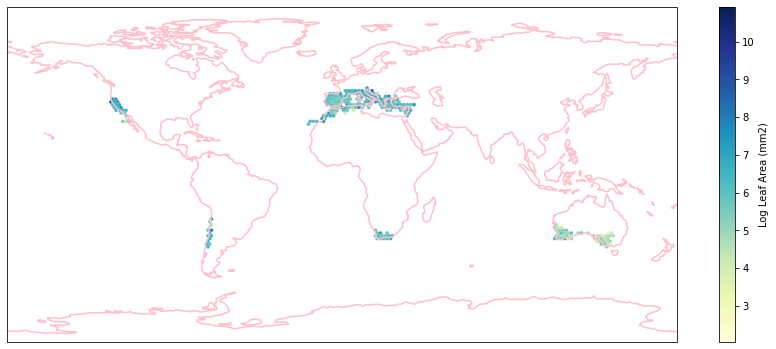
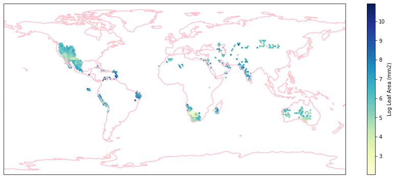
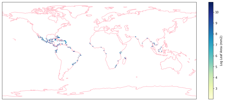
    df_merged.to_csv(filename, index=False)

Check work by plotting the different biomes:

for i in biome_types:

    # cut iNaturalist into a grid based on latitude and longitude
    iNat_with_biome_sub = iNat_with_biome[iNat_with_biome['BIOME']==i]
    
    fig = plt.figure(figsize=(15, 15))
    ax = plt.subplot(projection=ccrs.PlateCarree())
    ax.coastlines(resolution='110m', color='pink', linewidth=1.5)
    ax.set_extent([-180, 180, -90, 90], ccrs.PlateCarree())
    hb = ax.hexbin(iNat_with_biome_sub['decimalLongitude'], 
               iNat_with_biome_sub['decimalLatitude'], 
               C=iNat_with_biome_sub['Leaf Area'],
               reduce_C_function=np.mean,
               mincnt=1, 
               gridsize=(200, 60),
               cmap="YlGnBu", 
               transform=ccrs.PlateCarree(), 
               extent=[-180, 180, -90, 90],
               linewidths=0.1,
               vmin=iNat_TRY['Leaf Area'].quantile(0.01),
               vmax=iNat_TRY['Leaf Area'].quantile(0.99))
    cb = fig.colorbar(hb, ax=ax, shrink=0.41)
    cb.set_label('Log Leaf Area (mm2)')
    
    filename= "../Figures/biome_" + str(i) + "_leafarea.pdf"
    plt.savefig(filename, bbox_inches='tight')

Visualize differences in boxplot¶

List of biome names in the WWF data:

ID	Biome name
1	Tropical and subtropical moist broadleaf forests
2	Tropical and subtropical dry broadleaf forests
3	Tropical and subtropical coniferous forests
4	Temperate broadleaf and mixed forests
5	Temperate Coniferous Forest
6	Boreal forests / Taiga
7	Tropical and subtropical grasslands, savannas and shrublands
8	Temperate grasslands, savannas and shrublands
9	Flooded grasslands and savannas
10	Montane grasslands and shrublands
11	Tundra
12	Mediterranean Forests, woodlands and scrubs
13	Deserts and xeric shrublands
14	Mangroves

Aggregate forest biomes into the three main categories¶

Tropical and subtropical forests
Temperate forests
Boreal forests/Taiga


def agg_biome (row):
    if row['BIOME'] <= 3 :
        return 'Tropical and subtropical forests'
    if row['BIOME'] == 14 :
        return 'Mangroves'
    if row['BIOME'] == 9 :
        return 'Flooded grasslands and savannas'
    if row['BIOME'] == 7 :
        return 'Tropical and subtropical grasslands, savannas and shrublands'
    if row['BIOME'] == 13 :
        return 'Deserts and xeric shrublands'
    if row['BIOME'] == 12 :
        return 'Mediterranean Forests, woodlands and shrubs' 
    if row['BIOME'] == 8 :
        return 'Temperate grasslands, savannas and shrublands'
    if row['BIOME'] in range(4, 6) :
        return 'Temperate forests'
    if row['BIOME'] == 6 :
        return 'Boreal forests/Taiga'
    if row['BIOME'] == 10 :
        return 'Montane grasslands and shrublands'
    if row['BIOME'] == 11 :
        return 'Tundra'

# area and observations per biome
biome_types = [1.0,2.0,3.0,4.0,5.0,6.0,7.0,8.0,9.0,10.0,11.0,12.0,13.0,14.0]
biome_stats = pd.DataFrame(columns=["BIOME", "AREA", "iNat_Obs"])

for b in biome_types:
    biome_wwf = wwf[wwf['BIOME']==b]
    biome_area = biome_wwf['AREA'].sum()
    
    biome_iNat = iNat_with_biome[iNat_with_biome['BIOME']==b]
    biome_iNatobs = int(len(biome_iNat['BIOME']))
    biome_sPlot = sPlot_with_biome[sPlot_with_biome['BIOME']==b]
    biome_sPlotobs = int(len(biome_sPlot['BIOME']))
    
    df = pd.DataFrame([[b, biome_area, biome_iNatobs, biome_sPlotobs]], 
                      columns=["BIOME", "AREA", "iNat_Obs", "sPlot_Obs"])
    
    biome_stats = biome_stats.append(df)

# add biome name
biome_stats['AggBiome'] = biome_stats.apply (lambda row: agg_biome(row), axis=1)

# calculate observation density per square km

biome_stats['iNat_Density'] = biome_stats['iNat_Obs']/biome_stats['AREA']
biome_stats['sPlot_Density'] = biome_stats['sPlot_Obs']/biome_stats['AREA']

# obs ratio:

biome_stats['Obs_Ratio'] = biome_stats['iNat_Density']/biome_stats['sPlot_Density']

biome_stats

Aggregate different forest types¶

Aggregate tropical/temperate forest types and tropical/temperate grassland types

agg_biomes2 = biome_stats.groupby('AggBiome')['iNat_Obs'].sum()

agg_biomes1 = biome_stats.groupby('AggBiome', as_index =False)['AREA'].sum()
agg_biomes2 = biome_stats.groupby('AggBiome', as_index =False)['iNat_Obs'].sum()
agg_biomes = pd.concat([agg_biomes1, agg_biomes2["iNat_Obs"]], axis=1)

agg_biomes['Obs_Density'] = agg_biomes['iNat_Obs']/agg_biomes['AREA']
agg_biomes = agg_biomes.set_index('AggBiome')

agg_biomes

Normalize trait means¶

def quantile_norm(df, s1, s2, variables):
    
    # empty data frame to save output:
    df_norm = pd.DataFrame()
    
    for v in variables:
        
        # make subset df
        sub_exp = df[df['Trait']==v]
        sub_exp[s1] = np.exp(sub_exp[s1].copy())
        sub_exp[s2] = np.exp(sub_exp[s2].copy())
        
        # determine min and max values
        min_quantile = sub_exp[s1].quantile(0.05)
        max_quantile = sub_exp[s1].quantile(0.95)
        if min_quantile > sub_exp[s2].quantile(0.05):
            min_quantile = sub_exp[s2].quantile(0.05)
        if max_quantile < sub_exp[s2].quantile(0.95):
            max_quantile = sub_exp[s2].quantile(0.95)
      
        sub_exp[s1] = sub_exp[s1].apply(lambda x: (x - min_quantile)/(max_quantile - min_quantile))
        sub_exp[s2] = sub_exp[s2].apply(lambda x: (x - min_quantile)/(max_quantile - min_quantile))
        
        df_norm = pd.concat([df_norm, sub_exp])


    return df_norm

# init new df
raster_means_all = pd.DataFrame(columns=["x_bin","y_bin","Trait","TraitValue_sPlot","TraitValue_iNat","BIOME"])

for b in biome_types:
    filename="WWF/grid_means_biome" + str(b) + "_2deg.csv"
    raster_means = pd.read_csv(filename)
    
    # normalize trait measurements
    raster_means_biome = quantile_norm(raster_means, "TraitValue_sPlot", "TraitValue_iNat", trait)
    
    raster_means_biome['BIOME'] = b
    
    raster_means_all = pd.concat([raster_means_all, raster_means_biome])

Calculate difference between iNaturalist and sPlot maps (trait values all normalized):

raster_means_all['Difference'] = raster_means_all['TraitValue_iNat'] - raster_means_all['TraitValue_sPlot']

raster_means_all['AggBiome'] = raster_means_all.apply (lambda row: agg_biome(row), axis=1)

raster_means_all

raster_means_all.to_csv('raster_means_biomes_all_traits.csv', index=False)

Plot differences in boxplot¶

raster_means_all = pd.read_csv("raster_means_biomes_all_traits.csv")

def plot_boxplot(x, y, hue, data, xticklabels, xlabel, ylabel):
    
    sns.set_theme(style="white")
    
    colors = ['firebrick','cyan', 'slateblue', 'magenta','darkseagreen','pink','lavender']
    ax = sns.boxplot(x=x, 
                 y=y, 
                 hue=hue,
                 data=filtered_raster_means_all,
                 palette=colors,
                 showfliers = False,
                 #showmeans=True,
                 linewidth = 0.8,
                meanprops={"marker":"o","markerfacecolor":"white", "markeredgecolor":"blue"}
                )
    ax.set(xticklabels=xticklabels)


    plt.legend(ncol=7, loc='upper left')

    # add reference line at y=0
    ax.axhline(0, ls='--', linewidth=1, color='black')

    # rotate x-axis labels for readability 
    ax.set_xticklabels(ax.get_xticklabels(), rotation=50, ha="right")
    plt.ylabel(ylabel)
    plt.xlabel(xlabel)
    plt.tight_layout()

Plot Differences for top traits as boxplot:

value_list = ['Leaf Area', 'SLA', 
       'Leaf fresh mass', 'Leaf N per area', 'Plant Height',
       'Seed mass', 
       'Stem conduit density']

xticklabels =["Tropical and subtropical \n moist broadleaf forests",
              "Tropical and subtropical \n dry broadleaf forests",
              "Tropical and subtropical \n coniferous forests",
              "Temperate broadleaf \n and mixed forests",
              "Temperate Coniferous Forest", 
              "Boreal forests / Taiga",
              "Tropical and subtropical \n grasslands, savannas \n and shrublands",
              "Temperate grasslands, \n savannas and shrublands",
              "Flooded grasslands \n and savannas",
              "Montane grasslands \n and shrublands",
              "Tundra",
              "Mediterranean Forests, \n woodlands and shrubs",
              "Deserts and \n xeric shrublands","Mangroves"]


boolean_series = raster_means_all.Trait.isin(value_list)
filtered_raster_means_all = raster_means_all[boolean_series]

# set figure size
sns.set(rc={'figure.figsize':(15,9)})

# plot
plot_boxplot(x="BIOME",y="Difference", hue="Trait", data=filtered_raster_means_all, xticklabels=xticklabels,
             ylabel= "Scaled Difference (iNaturalist - sPlotOpen)", xlabel="Biome")

plt.savefig('../Figures/wwf_difference_all_7.pdf', bbox_inches='tight')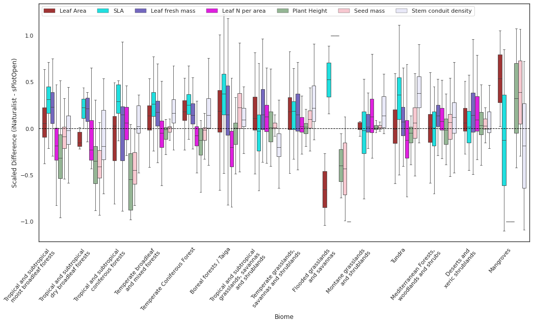

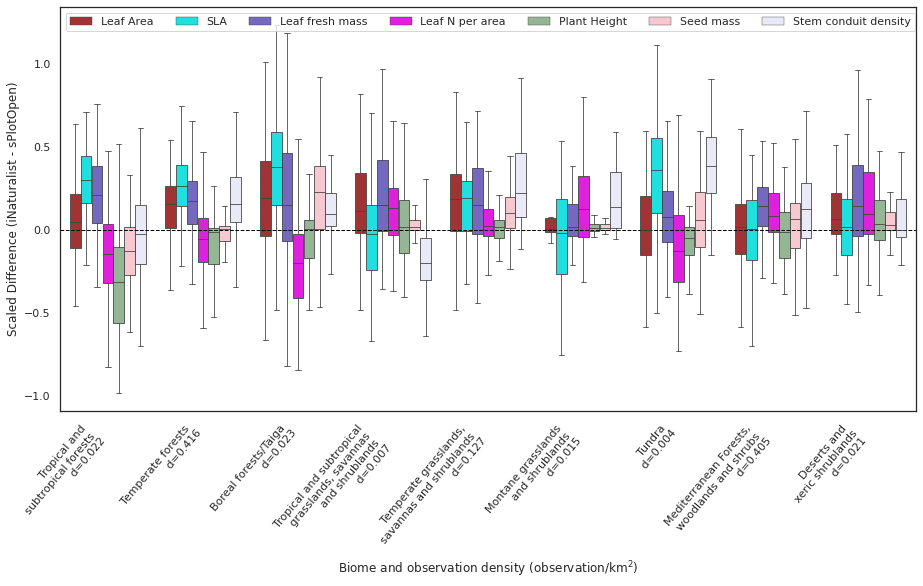
Aggregate the forests in to the 3 main categories:

# Difference
value_list = ['Leaf Area', 'SLA', 
       'Leaf fresh mass', 'Leaf N per area', 'Plant Height',
       'Seed mass', 
       'Stem conduit density']

xticklabels =["Tropical and \n subtropical forests \n d=" + 
              str(round(agg_biomes['Obs_Density'].loc[['Tropical and subtropical forests']][0], 3)),
              "Temperate forests \n d=" + 
              str(round(agg_biomes['Obs_Density'].loc[['Temperate forests']][0], 3)), 
              "Boreal forests/Taiga \n d=" + 
              str(round(agg_biomes['Obs_Density'].loc[['Boreal forests/Taiga']][0], 3)),
              "Tropical and subtropical \n grasslands, savannas \n and shrublands \n d=" + 
              str(round(agg_biomes['Obs_Density'].loc[['Tropical and subtropical grasslands, savannas and shrublands']][0], 3)),
              "Temperate grasslands, \n savannas and shrublands \n d=" + 
              str(round(agg_biomes['Obs_Density'].loc[['Temperate grasslands, savannas and shrublands']][0], 3)),
              "Montane grasslands \n and shrublands \n d=" + 
              str(round(agg_biomes['Obs_Density'].loc[['Montane grasslands and shrublands']][0], 3)),
              "Tundra \n d=" + 
              str(round(agg_biomes['Obs_Density'].loc[['Tundra']][0], 3)),
              "Mediterranean Forests, \n woodlands and shrubs \n d=" + 
              str(round(agg_biomes['Obs_Density'].loc[['Mediterranean Forests, woodlands and shrubs']][0], 3)),
              "Deserts and \n xeric shrublands\n d=" + 
              str(round(agg_biomes['Obs_Density'].loc[['Deserts and xeric shrublands']][0], 3))]

order = ["Tropical and subtropical forests",
        "Tropical and subtropical grasslands, savannas and shrublands",
        "Deserts and xeric shrublands",
        "Montane grasslands and shrublands",
        "Mediterranean Forests, woodlands and shrubs",
        "Temperate forests",
        "Temperate grasslands, savannas and shrublands",
        "Boreal forests/Taiga",
        "Tundra"]

boolean_series = raster_means_all.Trait.isin(value_list)
filtered_raster_means_all = raster_means_all[boolean_series]

boolean_series = filtered_raster_means_all.AggBiome.isin(order)
filtered_raster_means_all = filtered_raster_means_all[boolean_series]



# set figure size
sns.set(rc={'figure.figsize':(14,8.3)})

# plot
plot_boxplot(x="AggBiome",y="Difference", hue="Trait", data=filtered_raster_means_all, xticklabels=xticklabels, 
             xlabel = "Biome and observation density (observation/km$^2$)",
             ylabel = "Scaled Difference (iNaturalist - sPlotOpen)")


plt.savefig('../Figures/wwf_biomes_aggr_7.pdf', bbox_inches='tight', transparent=True)

Quantify average difference¶

raster_means_all = pd.read_csv("raster_means_biomes_all_traits.csv")

trait = ['Leaf Area', 'SLA', 
       'Leaf fresh mass', 'Leaf N per area', 'Plant Height',
       'Seed mass', 
       'Stem conduit density']

boolean_series = raster_means_all.Trait.isin(value_list)
filtered_raster_means_all = raster_means_all[boolean_series]

pd.set_option('display.max_rows', None)
medians= pd.DataFrame(filtered_raster_means_all.groupby(['AggBiome', 'Trait']).median()['Difference'])
medians.head()

medians = medians.reset_index(level=['AggBiome', 'Trait'])

Medians per trop trait in each biome:

medians = medians.pivot_table(index ='AggBiome', columns = 'Trait',
               values = 'Difference')

medians.loc["All Biomes"] = list(filtered_raster_means_all.groupby(['Trait']).median()['Difference'])
medians

medians = medians.round(2)

print(medians.to_latex(index=True))

\begin{tabular}{lrrrrrrr}
\toprule
Trait &  Leaf Area &  Leaf N per area &  Leaf fresh mass &  Plant Height &   SLA &  Seed mass &  Stem conduit density \\
AggBiome                                           &            &                  &                  &               &       &            &                       \\
\midrule
Boreal forests/Taiga                               &       0.19 &            -0.20 &             0.15 &          0.01 &  0.38 &       0.22 &                  0.09 \\
Deserts and xeric shrublands                       &       0.06 &             0.09 &             0.14 &          0.04 &  0.02 &       0.03 &                 -0.00 \\
Flooded grasslands and savannas                    &      -0.65 &             1.00 &             1.00 &         -0.40 &  0.53 &      -0.43 &                 -1.00 \\
Mangroves                                          &       0.54 &            -1.00 &            -1.00 &          0.33 & -0.12 &       0.39 &                 -0.18 \\
Mediterranean Forests, woodlands and shrubs        &       0.02 &             0.08 &             0.14 &         -0.01 &  0.01 &       0.06 &                  0.12 \\
Montane grasslands and shrublands                  &       0.01 &             0.13 &             0.02 &          0.01 & -0.02 &       0.01 &                  0.14 \\
Temperate forests                                  &       0.15 &            -0.06 &             0.18 &         -0.02 &  0.26 &       0.00 &                  0.15 \\
Temperate grasslands, savannas and shrublands      &       0.18 &             0.02 &             0.15 &          0.02 &  0.19 &       0.10 &                  0.22 \\
Tropical and subtropical forests                   &       0.05 &            -0.15 &             0.21 &         -0.32 &  0.30 &      -0.13 &                 -0.03 \\
Tropical and subtropical grasslands, savannas a... &       0.11 &             0.13 &             0.15 &          0.01 & -0.03 &       0.01 &                 -0.20 \\
Tundra                                             &      -0.00 &            -0.13 &             0.08 &         -0.05 &  0.36 &       0.06 &                  0.38 \\
All Biomes                                         &       0.11 &            -0.02 &             0.15 &         -0.01 &  0.20 &       0.01 &                  0.11 \\
\bottomrule
\end{tabular}