Calculate correlation of sPlot CWM and iNaturalist averages
Here we correlate the aggregated trait values close each sPlot (with a certain range) to the community weighted trait mean of each plot (cwm).
This section includes:
Plot r for each buffer size
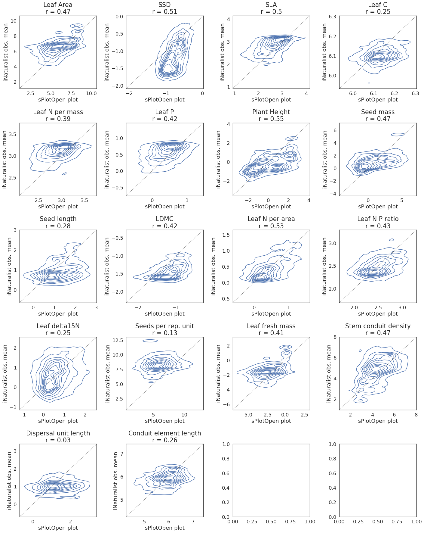
Scatter correlation plots for 64,000 m buffer size
import pandas as pd
import numpy as np
import os

#plotting
import matplotlib.pyplot as plt
import seaborn as sns
from matplotlib.colors import LogNorm, Normalize
import cartopy.crs as ccrs
from matplotlib.colors import BoundaryNorm
from matplotlib.ticker import MaxNLocator

import math
sPlot = pd.read_csv("sPlotOpen/cwm_loc.csv")Plot r for each buffer size
buffer_sizes = [1000,2000,4000,8000,16000,32000,64000,128000,256000]

trait =['Leaf Area',
 'SSD',
 'SLA',
 'Leaf C',
 'Leaf N per mass',
 'Leaf P',
 'Plant Height',
 'Seed mass',
 'Seed length',
 'LDMC',
 'Leaf N per area',
 'Leaf N P ratio',
 'Leaf delta15N',
 'Seeds per rep. unit',
 'Leaf fresh mass',
 'Stem conduit density',
 'Dispersal unit length',
 'Conduit element length'
       ]

r_all = pd.DataFrame(columns=trait)


for buffer in buffer_sizes:

    file_name = "Buffer_Rerun/all_buffer_means_" + str(buffer) + ".csv"
    buffer_means = pd.read_csv(file_name,
                          sep=",",
                          usecols=['NumberiNatObservations','PlotObservationID', 'Leaf Area',
                                   'SSD',
 'SLA',
 'Leaf C',
 'Leaf N per mass',
 'Leaf P',
 'Plant Height',
 'Seed mass',
 'Seed length',
 'LDMC',
 'Leaf N per area',
 'Leaf N P ratio',
 'Leaf delta15N',
 'Seeds per rep. unit',
 'Leaf fresh mass',
 'Stem conduit density',
 'Dispersal unit length',
 'Conduit element length'
                                  ],
                          index_col=False)

    buffer_means = buffer_means[~buffer_means.isin([np.nan, np.inf, -np.inf]).any(1)]
    #transform dataframe from wide to long

    sPlot_t = sPlot.melt(id_vars=["PlotObservationID", "Latitude", "Longitude", "Biome", "Naturalness", "Forest",
                              "Shrubland", "Grassland", "Wetland", "Sparse_vegetation"],
                     value_name="TraitValue",
                     var_name="Trait",
                     value_vars=trait)

    buffer_means_t = buffer_means.melt(id_vars=["PlotObservationID", "NumberiNatObservations"],
                                   value_name="TraitValue",
                                   var_name="Trait",
                                   value_vars=trait)

    sPlot_buffers_merged = pd.merge(sPlot_t, buffer_means_t, on=["PlotObservationID", "Trait"])


    # claculate r and ranges for all traits

    r_buffer=[]

    for i in trait:
        #corr_trait = sPlot[i].fillna(0).corr(buffer_means[i].fillna(0))
        corr_trait = sPlot[i].corr(buffer_means[i])
        r_trait = corr_trait
        r_buffer.append(r_trait)

    s = pd.Series(r_buffer, index=r_all.columns)
    r_all = r_all.append(s, ignore_index=True)


r_all['BufferSize'] = buffer_sizesr_allLoading...
# https://stackoverflow.com/questions/44941082/plot-multiple-columns-of-pandas-dataframe-using-seaborn
# https://lost-stats.github.io/Presentation/Figures/line_graph_with_labels_at_the_beginning_or_end.html

# data
data_dropnan = r_all.dropna(axis=1, how='all')
data_melt=pd.melt(data_dropnan, ['BufferSize'], value_name="r")
data_melt =data_melt.astype({"BufferSize": str}, errors='raise')

# label names
trait_names = data_melt["variable"].unique()

sns.set(rc={'figure.figsize':(8,10)})
sns.set_theme(style="white")
fig, ax = plt.subplots()

# plot all lines into one plot

sns.lineplot(x='BufferSize',
            y='r',
            hue='variable',
            data=data_melt,
            ax=ax,
            marker='o',
            legend=None,
            linewidth=0.6)

label_pos=[]

# Add the text--for each line, find the end, annotate it with a label
for line, variable in zip(ax.lines, trait_names):
    y = line.get_ydata()[-1]
    x = line.get_xdata()[-1]
    if not np.isfinite(y):
        y=next(reversed(line.get_ydata()[~line.get_ydata().mask]),float("nan"))
    if not np.isfinite(y) or not np.isfinite(x):
        continue
    x=round(x)
    y=round(y,2)
    xy=(x*1.02, y)
    if xy in label_pos:
        xy=(x*1.02, y-0.01)
    if xy in label_pos:
        xy=(x*1.02, y+0.01)
    label_pos.append(xy)
    text = ax.annotate(variable,
                       xy=(xy),
                       xytext=(0, 0),
                       color=line.get_color(),
                       xycoords=(ax.get_xaxis_transform(),
                                 ax.get_yaxis_transform()),
                       textcoords="offset points")
    text_width = (text.get_window_extent(
    fig.canvas.get_renderer()).transformed(ax.transData.inverted()).width)
    #if np.isfinite(text_width):
     #   ax.set_xlim(ax.get_xlim()[0], text.xy[0] + text_width * 1.05)

# Format the date axis to be prettier.
sns.despine()
plt.xlabel("Buffer Size in meters")
plt.ylabel("r")
plt.tight_layout()

plt.savefig('../Figures/r_buffer.pdf', bbox_inches='tight') 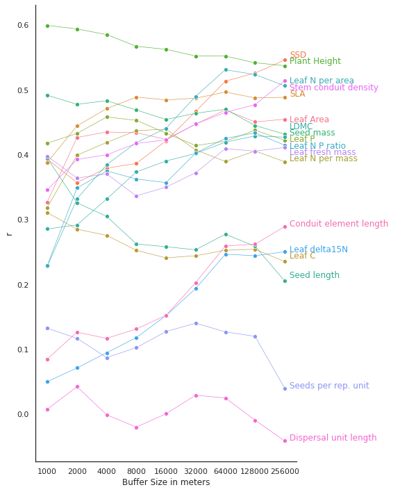
Scatter correlation plots for 64,000 m buffer size
optimal_buffer_size = 64000
file_name = "Buffer_Rerun/all_buffer_means_" + str(optimal_buffer_size) + ".csv"
buffer_means = pd.read_csv(file_name,
                          sep=",",
                          usecols=['NumberiNatObservations','PlotObservationID', 'Leaf Area',
                                   'SSD',
 'SLA',
 'Leaf C',
 'Leaf N per mass',
 'Leaf P',
 'Plant Height',
 'Seed mass',
 'Seed length',
 'LDMC',
 'Leaf N per area',
 'Leaf N P ratio',
 'Leaf delta15N',
 'Seeds per rep. unit',
 'Leaf fresh mass',
 'Stem conduit density',
 'Dispersal unit length',
 'Conduit element length'
                                  ],
                          index_col=False)
buffer_means = buffer_means[~buffer_means.isin([np.nan, np.inf, -np.inf]).any(1)]
#transform dataframe from wide to long
sPlot_t = sPlot.melt(id_vars=["PlotObservationID", "Latitude", "Longitude", "Biome", "Naturalness", "Forest",
"Shrubland", "Grassland", "Wetland", "Sparse_vegetation"],
value_name="TraitValue",
var_name="Trait",
value_vars=trait)
buffer_means_t = buffer_means.melt(id_vars=["PlotObservationID", "NumberiNatObservations"],
value_name="TraitValue",
var_name="Trait",
value_vars=trait)
sPlot_buffers_merged = pd.merge(sPlot_t, buffer_means_t, on=["PlotObservationID", "Trait"])trait=['Leaf Area',
'SSD',
'SLA',
'Leaf C',
'Leaf N per mass',
'Leaf P',
'Plant Height',
'Seed mass',
'Seed length',
'LDMC',
'Leaf N per area',
'Leaf N P ratio',
'Leaf delta15N',
'Seeds per rep. unit',
'Leaf fresh mass',
'Stem conduit density',
'Dispersal unit length',
'Conduit element length']
# calculate max-min ranges

def min__max_ranges(df, col_1, col_2, variable_col, variables):

    range_all =[]

    for i in variables:
        df_sub = df[df[variable_col]==i]
        df_sub = df_sub.dropna(subset = [col_1, col_2])

        xmin = df_sub[col_1].quantile(0.01)
        xmax = df_sub[col_1].quantile(0.99)

        ymin = df_sub[col_2].quantile(0.01)
        ymax = df_sub[col_2].quantile(0.99)


        if xmin>ymin:
            if not np.isfinite(ymin):
                pass
            else:
                xmin = ymin
        else:
            pass

        if xmax<ymax:
            xmax=ymax
        else:
            pass

        range_sub = [xmin, xmax]

        range_all.append(range_sub)

    ranges  = pd.DataFrame()
    ranges['variable'] = variables
    ranges['min'] = [i[0] for i in range_all]
    ranges['max'] = [i[1] for i in range_all]
    ranges = ranges.set_index('variable')

    return ranges
ranges = min__max_ranges(sPlot_buffers_merged, 'TraitValue_x', 'TraitValue_y',
variable_col='Trait', variables=trait)rangesLoading...
This might take a few minutes to plot:
fig, axes = plt.subplots(ncols=4, nrows=5, figsize=(20,25))

sns.set_theme(style="white", font_scale=1.7)

for i, ax in zip(trait, axes.flat):

    sub_df = sPlot_buffers_merged[sPlot_buffers_merged["Trait"]==i]

    index=0
    trait_title= str(i) + "\n" + "r = " + str(round(r_all.loc[6, i], 2))

    sns.kdeplot(
        data=sub_df,
        x="TraitValue_x",
        y="TraitValue_y",
        ax=ax,
        ).set(title=trait_title, xlabel='sPlotOpen plot', ylabel='iNaturalist obs. mean')

    ax.axline([0, 0], [1, 1], color= "black", alpha=0.6, ls = ":")

    space = (ranges.loc[i, "max"]-[ranges.loc[i, "min"]]) * 0.2
    ax.set_xlim(ranges.loc[i, "min"] - abs(space), ranges.loc[i, "max"] + abs(space))
    ax.set_ylim(ranges.loc[i, "min"] - abs(space), ranges.loc[i, "max"] + abs(space))

    index+=1

fig.tight_layout()

plt.savefig('../Figures/corr_buffer_all_64k_kde.pdf', bbox_inches='tight')